Tomography

The principle of computed tomography (CT) is to acquire a large number of x-rays all around the object, such so as to measure for each orientation the x-ray image in that direction. From this set of x-ray projections, the reconstruction allows us to get a 3D image of this linear attenuation coefficient.

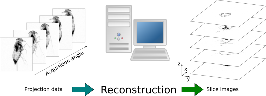
Fig. 141 Tomographic reconstruction

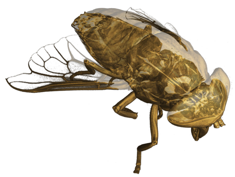
Fig. 142 3D rendering of the fly (neutron CT)

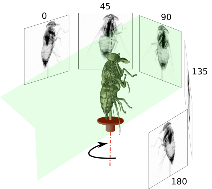
Fig. 143 Tomographic acquisition (circular trajectory). From PSI

The reconstruction algorithm requires as input for each pixel of each projection an integral of the 3D scalar value. For the x-ray acquisition, this 3D scalar value to be reconstructed for each voxel \(v\) is simply the attenuation coefficient \(\mu\). Recalling the Beer-Lambert law (see section Attenuation law), we have one equation per pixel \(p\) as follows:

\[ \ln \frac{I_0(p)}{I(p)} = \int_{v\in \mathsf{ray}(p)} \mu(v) \mathsf{d}v \]

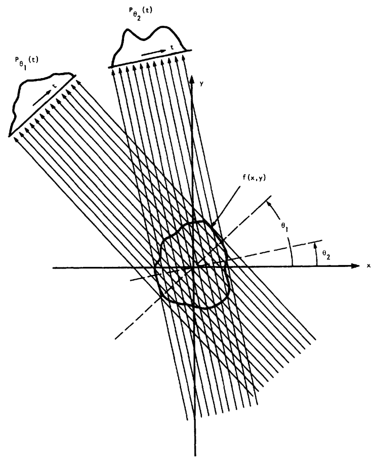
Fig. 144 Tomography: relationship with the Beer-Lambert attenuation law. From Kak & Slaney

Suppose we have a flat-panel detector of \(N_X \times N_Y\) pixels and suppose we acquire \(N_P\) x-ray projections around the object, the number of integral data we get is simply \(N_X \times N_Y \times N_P\) which can be huge for standard imaging devices. To solve this inverse problem there are analytical methods (which solve the integral in the continuous domain before spatial discretization) and algebraic methods (which discretize the problem in the matrix form \(Ax=b\) before solving it). See for more details the book of Kak & Slaney available

This set of \(N_X \times N_Y \times N_P\) line integrals is known as the sinogram or Radon tranform. The name sinogram can easily be understood if we look at the same detecteor line in terms of the rotation angle. Fig. 147 shows such an image and the sine shape is clearly visible.

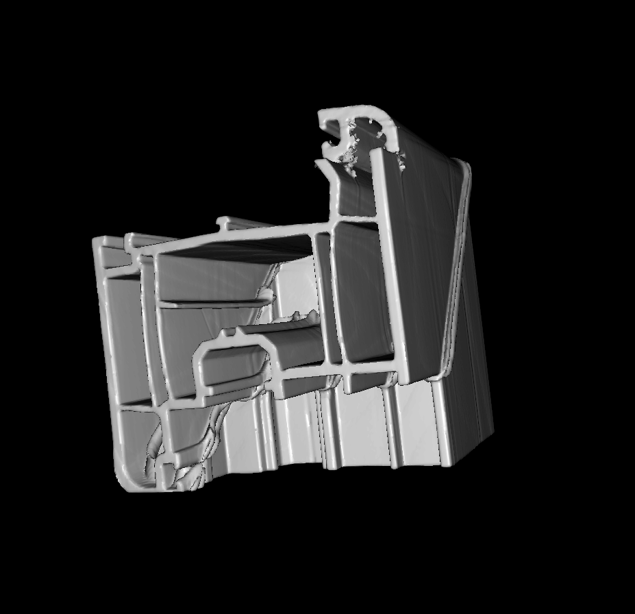
Fig. 145 3D surface rendering of a PVC window part

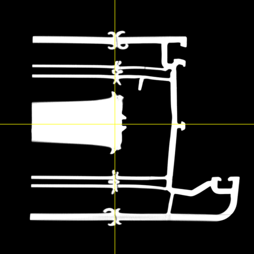
Fig. 146 A slice in the reconstructed volume of a PVC window part

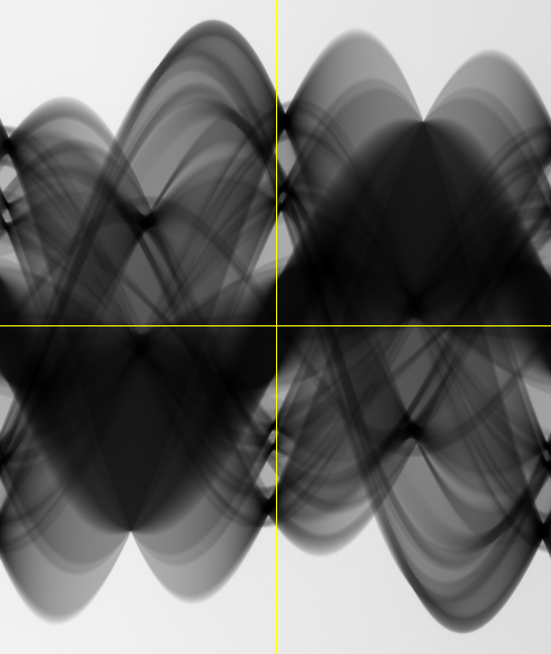
Fig. 147 Sinogram of a PVC window part. The vertical axis is the intensity profile sampled for the same detector line, ad the horizontal axis is the projection angle.

The most basic reconstruction is the simple back projection of the measured values ​​along the rays. The resulting 3D image is blurry. An analytical model image formation shows that it is necessary to make a ramp filter in the Fourier domain before backproject to have an exact reconstructed 3D image.

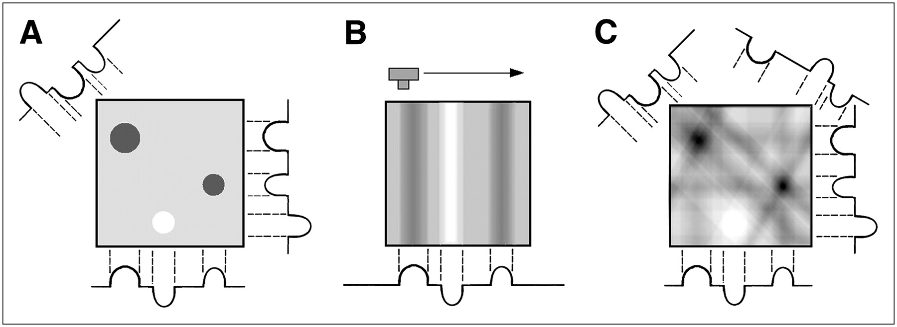
Fig. 148 Backprojection. Original object (left), backprojection of the line integrals from a single x-ray projection (middle), and backprojection of the line integrals from four x-ray projections (right)

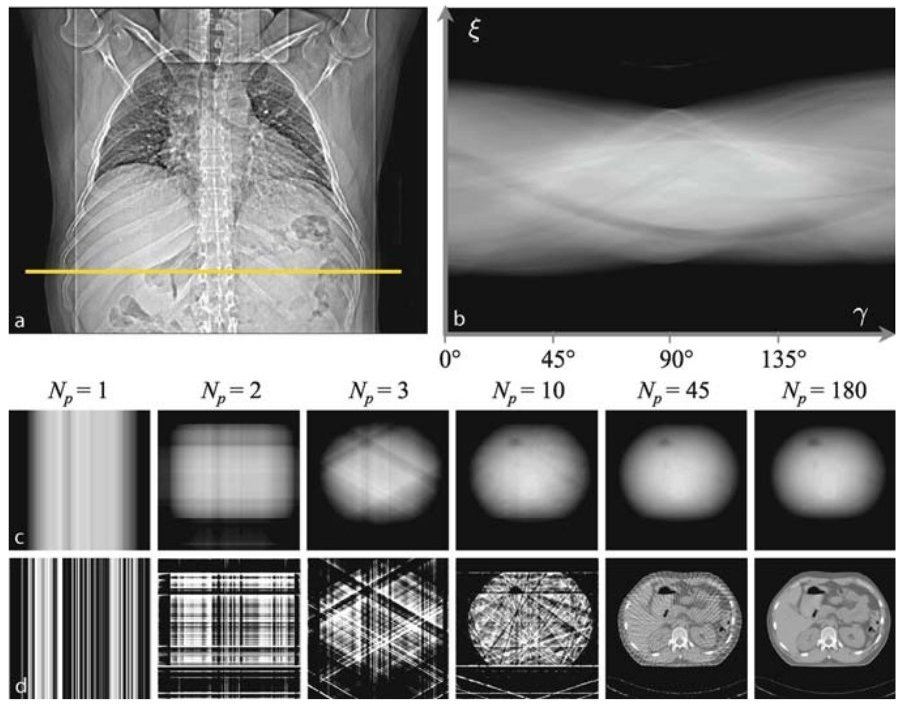
Fig. 149 Filtered Backprojection (FBP) vs Backprojection (BP). Successive reconstruction of a tomographic abdomen image from projection data. Image a shows the position of the axial abdomen section in a planning overview. In image b the corresponding sinogram, i.e., the complete Radon space data of the sectional plane, can be seen. Column-wise the simple backprojections (row c) and the corresponding filtered backprojections (row d) are presented for the increasing projection numbers. From Buzug DOI

The circular trajectory does not allow reconstruction in a way exact as in the plan of acquisition. The acquisition in helical mode allows for a more accurate reconstruction.

Fig. 150 A necessary condition for exact reconstruction is that for every plane that intersects the object there exists at least one cone-beam source point

Some examples of sinograms and reconstructed volumes are given in the following.

Fig. 151 Chest sinogram.

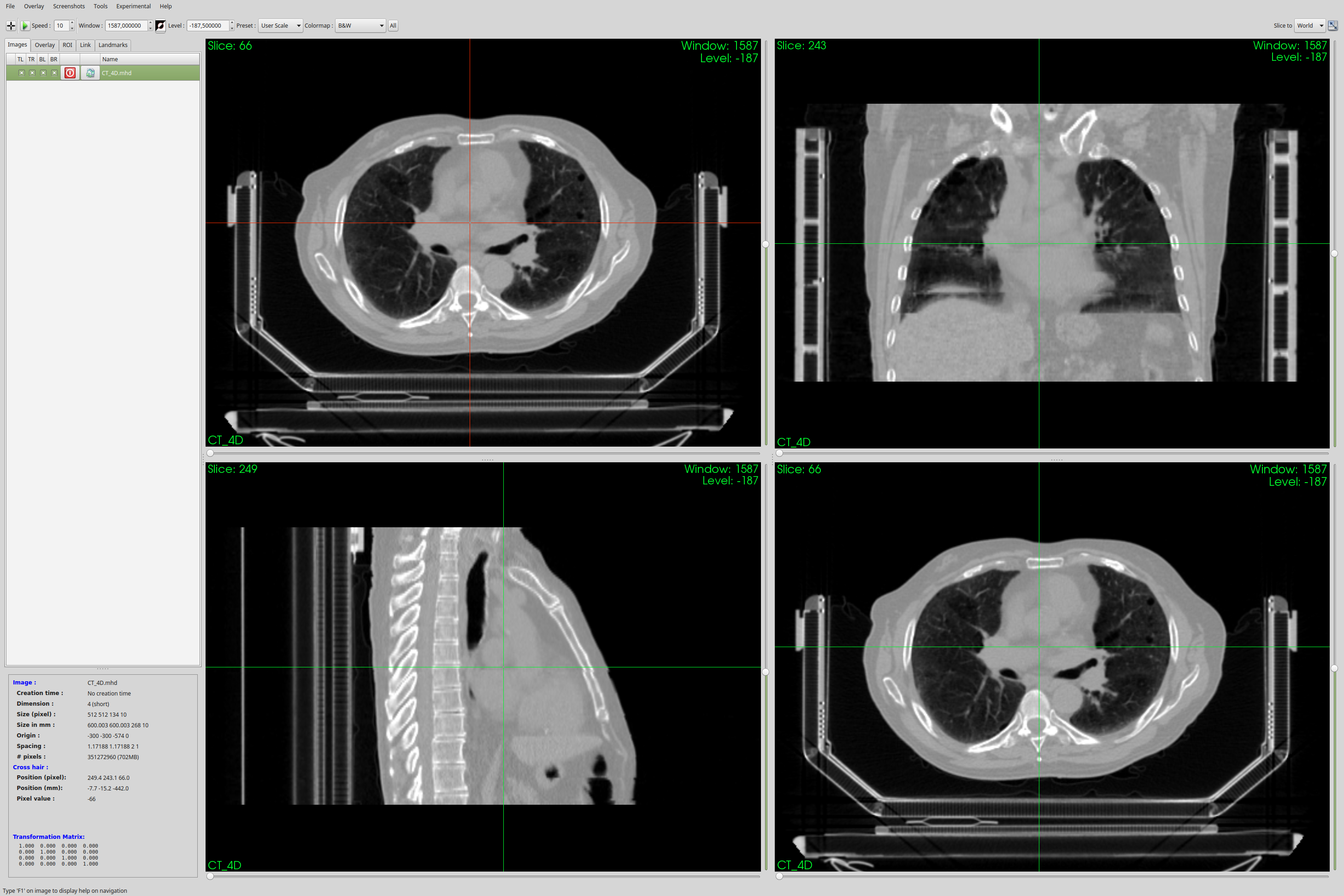
Fig. 152 Orthoviews of the reconstructed chest volume

An example in NDT.

Fig. 153 Legoman sinogram.

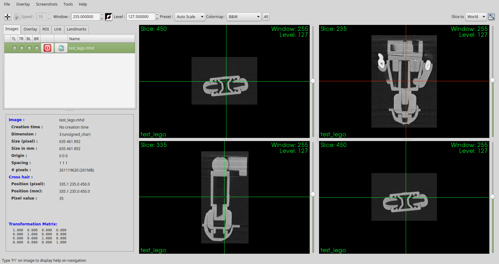
Fig. 154 Orthoviews of a reconstructed Legoman volume.

Tomographic setup combining rotation and translation: helical mode. This mode is particularly suitable for long objects.

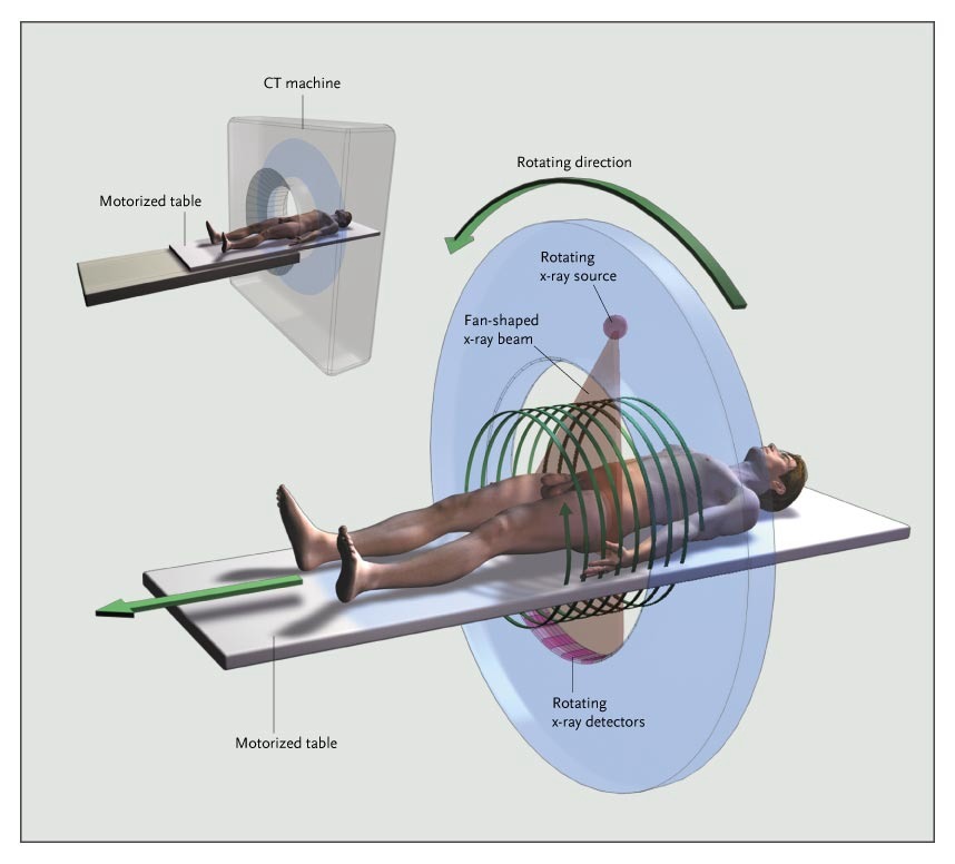
Fig. 155 Acquisition in helical mode.

Tomographic setup with source motion parallel to the detector plane: Tomosynthesis or Laminography mode. This mode is interesting for flat cumbersome objects.

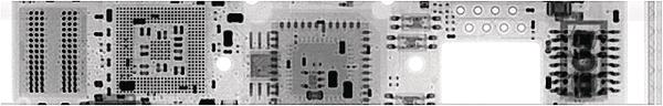
Fig. 156 PCB solder joint inspection: Standard 2D RX

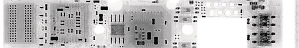
Fig. 157 PCB solder joint inspection: Laminography, top layer

Fig. 158 PCB solder joint inspection: Laminography, bottom layer

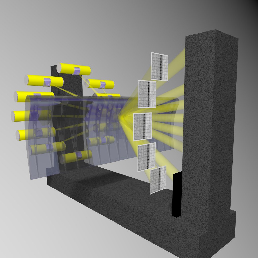
Fig. 159 Acquisition in tomosynthesis (aka laminography) mode.

The presence of secondary radiation (scattered) is particularly important in conical beams because the object is fully irradiated. On the other hand the fan beam geometry (with a detector linear) very strongly limits the presence of secondary radiation on the detector. These scattered radiation can greatly degrade the image 3D reconstructed: it is not quantitatively exploitable. Technological solutions (eg with an anti-scatter grid) and methodologies (eg with an air-gap or a beam-stop array) exist to reduce the impact of this scattered radiation.

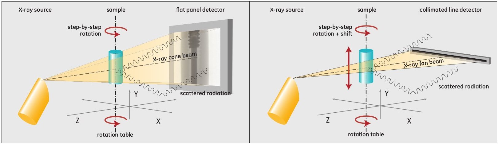
Fig. 160 Scatter: Fan-beam vs Cone-beam acquisition setup. Conventional cone beam CT with scattered radiation hitting the detector (left). Scatter artifact reduced slice-by-slice fan beam CT (right)

An example of use of a beam-stop array (BSA) to compute and reduce the x-ray scatter contribution.

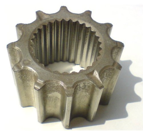
Fig. 161 Sintered powder sample (iron)

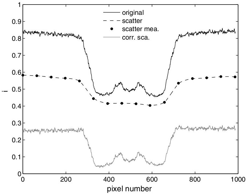
Fig. 162 Intensity profiles in the projection images.

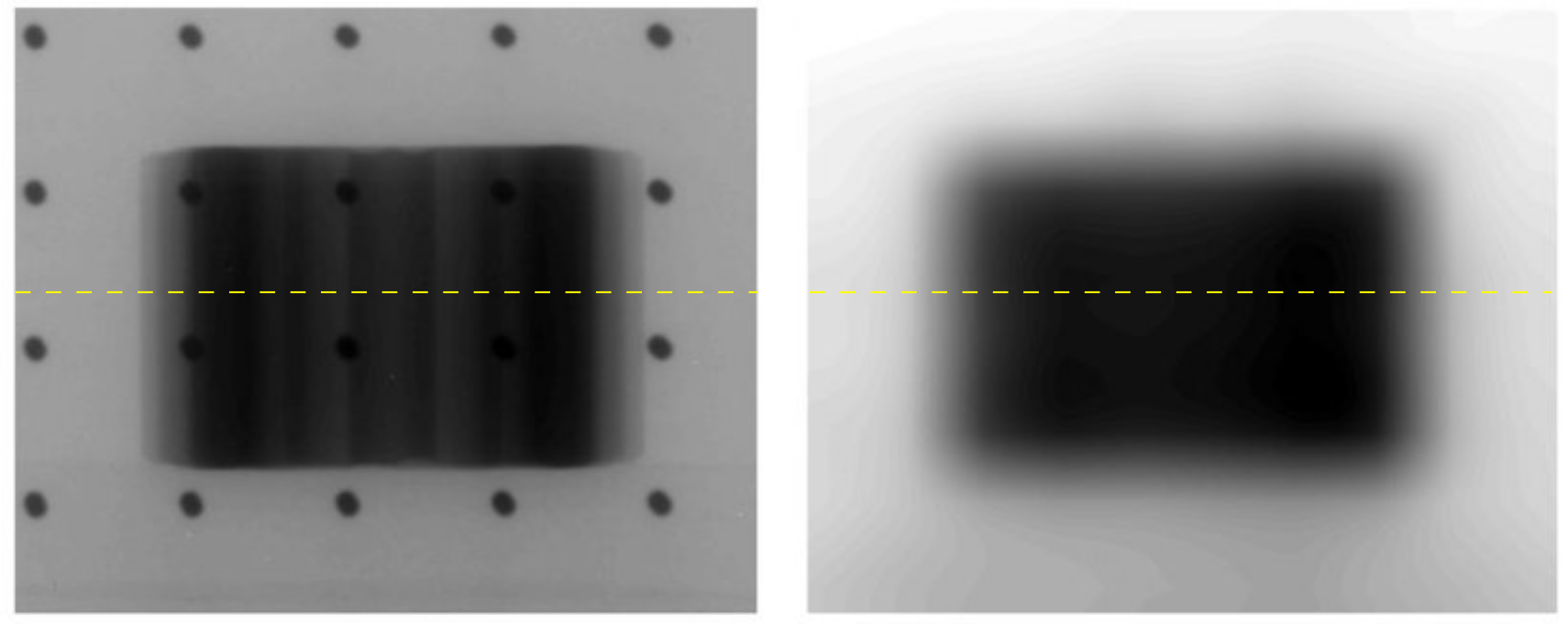
Fig. 163 400 kV acquisition (left) and BSA scatter estimation (right). In dashed lines the profiles in Fig. 162

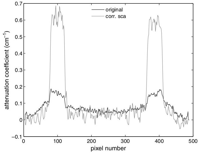
Fig. 164 Intensity profiles in the reconstruction images.

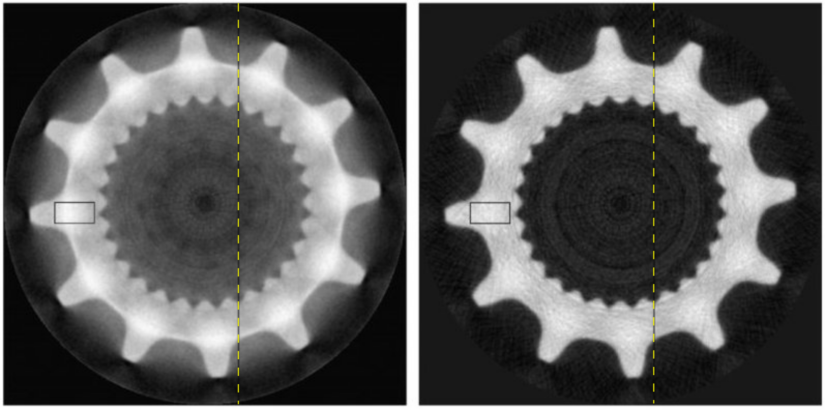
Fig. 165 Slice of the recontructed volume: Raw FBP reconstruction (left), Scatter-corrected FBP reconstruction (right). From Peterzom NIMB 2008 DOI

Some NDT applications of tomography taken from GrabCAD:

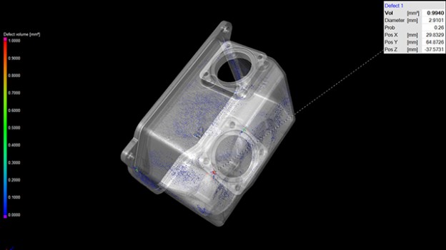
Fig. 166 Void analysis: inspecting for internal voids or inclusions within a part. See video

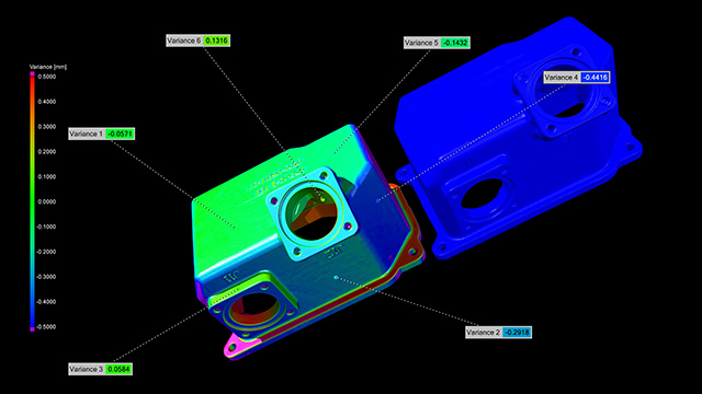
Fig. 167 Part to CAD comparison inspecting the part by comparing it to the CAD model. See video

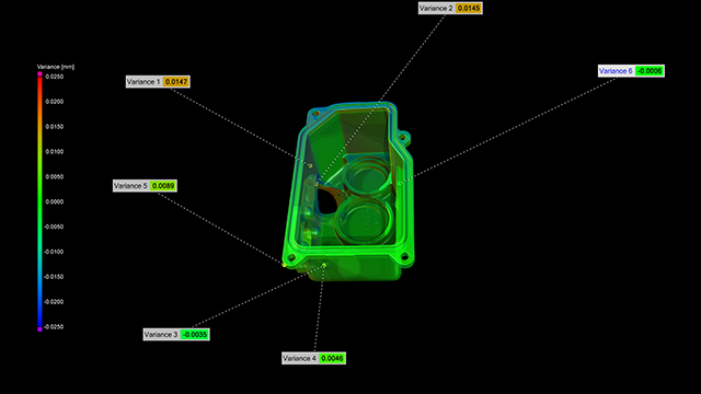
Fig. 168 Part to part comparison: inspecting two parts and comparing them to each other. See video

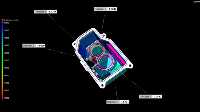
Fig. 169 Wall thickness analysis inspecting consistencies in a parts wall structure. See video

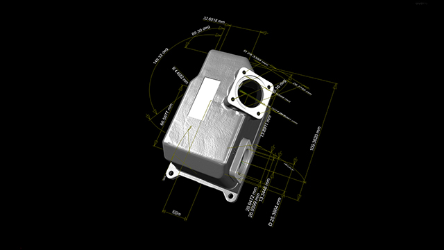
Fig. 170 First article inspection geometric dimensioning and tolerancing (GD&T). See video

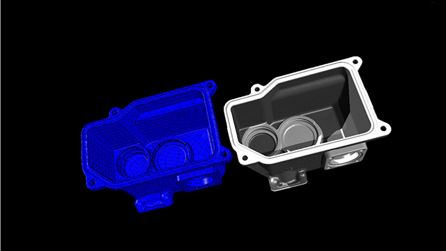
Fig. 171 Reverse engineering: development a CAD file \(\Rightarrow\) 3D printing. See video

• Void analysis in Fig. 166

• Part to CAD comparison in Fig. 167

• Part to part comparison in Fig. 168

• Wall thickness analysis in Fig. 169

• First article inspection in Fig. 170

• Reverse engineering in Fig. 171

Dual-energy tomography can separate several phases according to their difference in attenuation.

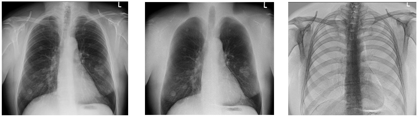
Fig. 172 Standard radiography (left). Dual-energy radiography decomposition: soft tissue component (middle) and bone component (right)

Fig. 173 Dual-energy CT: Homeland security. See video

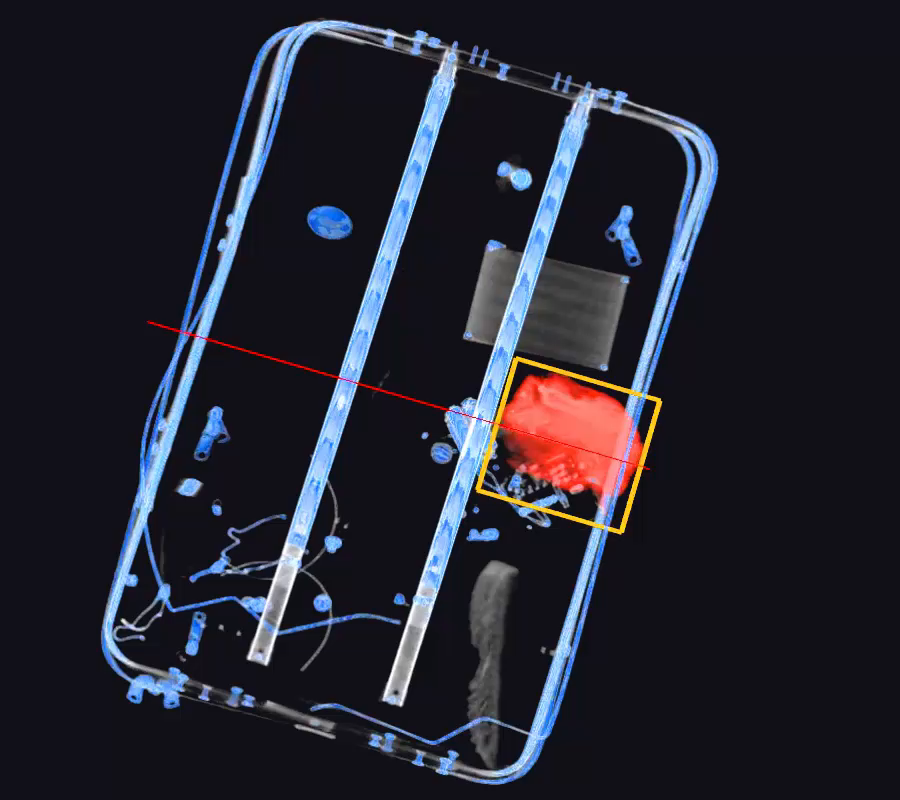
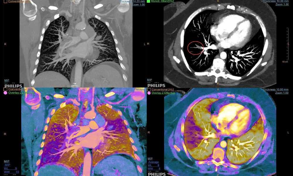
Fig. 174 “Color” tomography (Effective Z map) by a prototype medical scanner with an energy-resolved detector from Philips IQon Spectral CT. Functional imaging with tracers is now possible with spectral x-ray tomography.

Comparison of attenuation and phase imagery of a aluminum-silicon alloy. The sensitivity of the imaging phase to density differences is much more important.

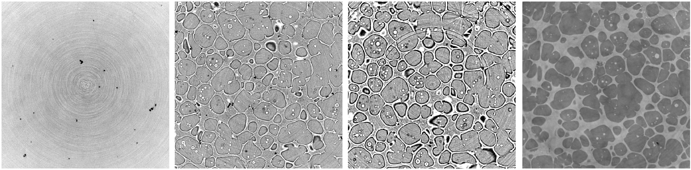
Fig. 175 Phase imaging (from JY Buffière): Al-Si alloy (ROI 1mm). Slices of standard x-ray attenuation reconstructed volumes with increasing sample-to-detector distance: 3 mm (left), 200 mm (middle left), and 500 mm (middle right). Phase contrast fringes appear. Reconstructed phase volume (right). The phase component is much more sensitive to density changes than the attenuation component (see Fig. 73 in section Wave).