Instrumentation

X-ray production

Energy distribution

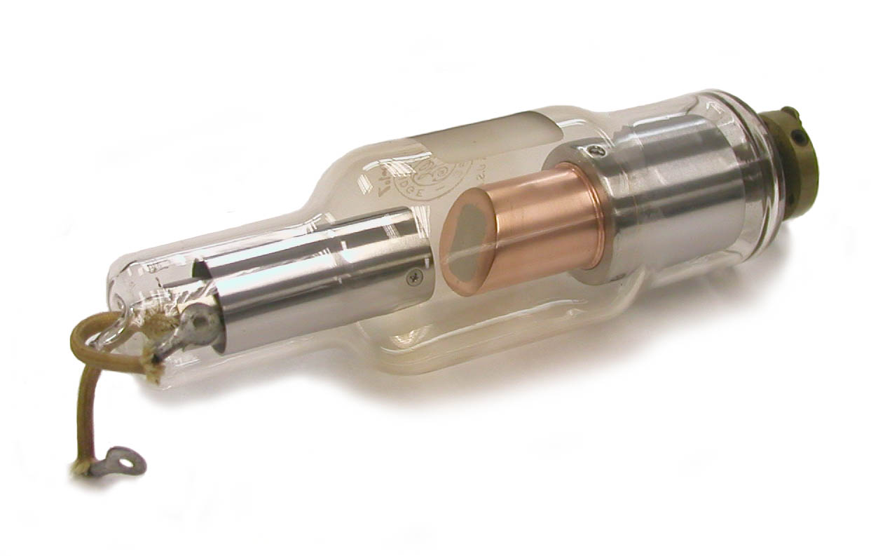
Fig. 83 Old X-ray tube (glass wall chamber)

Fig. 84 X-ray tube principle: William Coolidge in 1913}

The principle of an x-ray tube is the following. Electrons in a heated filament, with a current of a few mA typically, are extracted using a very high voltage \(U\) (several tens of kV typically). Their kinetic energy is close to 0 in the filament (they can be considered at rest). Therefore their kinetic energy reach \(U\) keV just before impinging onto the anode target. From electron-matter interactions in the target follow X-ray mostly produced by Bremsstrahlung but also to a lesser extent Fluorescence. Refer to section Electron-matter interactions.

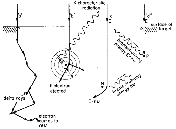
Fig. 85 Typical electron interactions with a target. (a) Electron suffers ionizational losses, giving rise to heat. (b) The electron ejects a K electron giving rise to Fluorescence. (c) Collision between an electron and a nucleus. (d) Rare collision when the electron is completely stopped in one collision. From Johns DOI

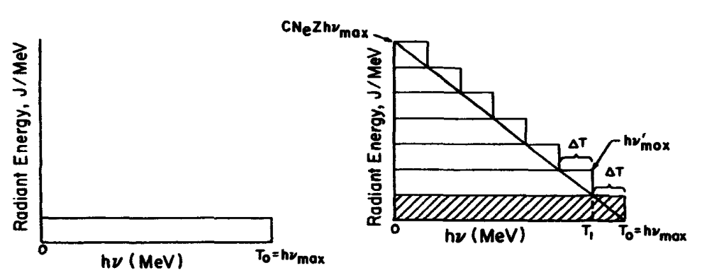
Fig. 86 Bremsstrahlung radiant-energy spectrum from a thin target (left) and a thick target (right). From Attix DOI

A monoenergetic electron beam impacting a target thin metal produces a uniform energy spectrum of Bremsstrahlung x-rays. For a thick anode, the radiant-energy spectrum of emitted photons is a function linearly decreasing.

Fig. 87 Classical explanation of the thin-target x-ray spectrum generated by nonrelativistic electrons. From Attix DOI

Thin-target model of the radiant-energy spectrum (excerpt from Attix DOI):

Consider a beam of electrons of kinetic energy \(T_o\) entering the page perpendicularly, and each passing the nucleus at some distance (impact parameter) \(b\) (see section Electron-matter interactions). The differential interaction cross-section when \(b = b_1\) is proportional to the area \(dA_1 = 2\pi b_1 db\). For \(b_2 = 2b_1\), \(dA_2 = 2 dA_1\). Thus twice as many photons \(N_2\) come from interactions in \(dA_2\), as the \(N_1\) from \(dA_1\). If the magnitude of the interaction (i.e., the x-ray quantum energy \(hv\) produced) is assumed to be proportional to \(1/b\), then \(hv_1 = 2 hv_2\), Therefore \(N_1hv_1 = N_2hv_2\), and the x-ray radiant-energy spectrum should be flat, as it is observed to be.

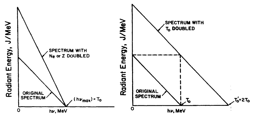
Fig. 88 Influence of current and voltage on the x-ray radiant-energy spectrum

The high voltage accelerating electrons conditions the maximum energy value of the emitted photons, while the current only changes the photon rate without modify the maximum value.

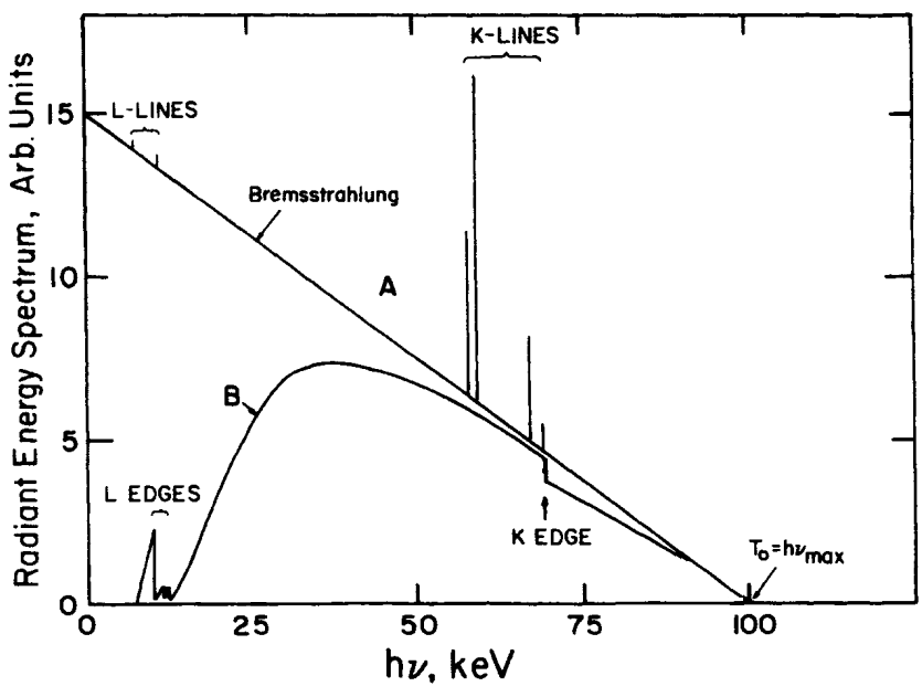
Fig. 89 X-ray spectrum from 100-keV electrons on a thick tungsten target. Upper curve A: Unfiltered. B: Filtered through \(0.01\) mm W in escaping the anode target. To avoid confusion, the K-fluorescence lines are not shown in curve B, but are attenuated from their heights in curve A in the same proportion as the Bremsstrahlung is attenuated at the same energies. From Attix DOI

The linear coefficient of the materials being more important at low energies, the spectrum exiting the anode target no longer has its low-energy components (spectrum B of Fig. 89).

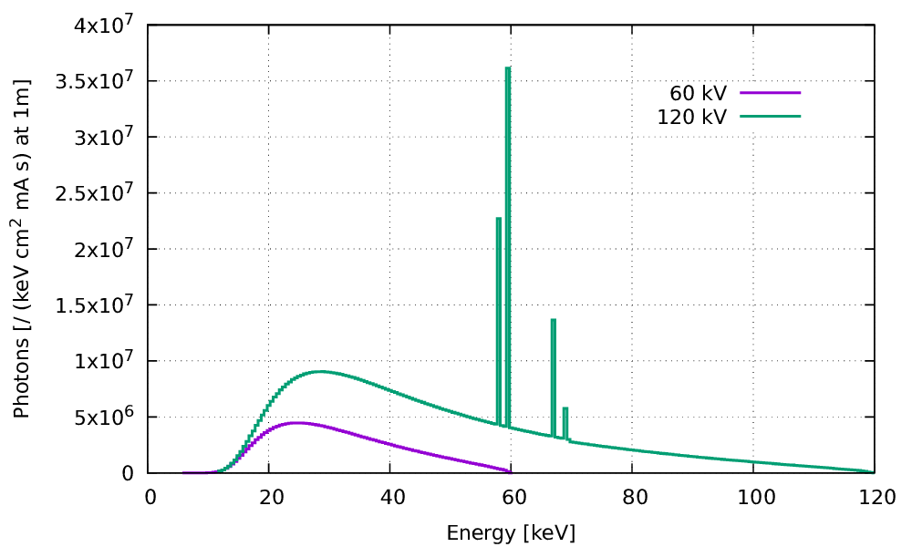
Fig. 90 X-ray spectrum (in photon counts not radian energy): Influence of mA and kV

X-ray spectra emitted at 60 and 120 kV high voltage. We sees the characteristic lines of the anode fluorescence in tungsten following ionizations by the electron beam.

Beam hardening

When x-rays pass through matter, the low-energy components are more attenuated than the high-energy ones because the linear attenuation coefficient globally decreases when the photon energy is increased. Figure Fig. 91 shows how a 60kV x-ray spectrum is affected by a 150-micron-thick cupper foil.

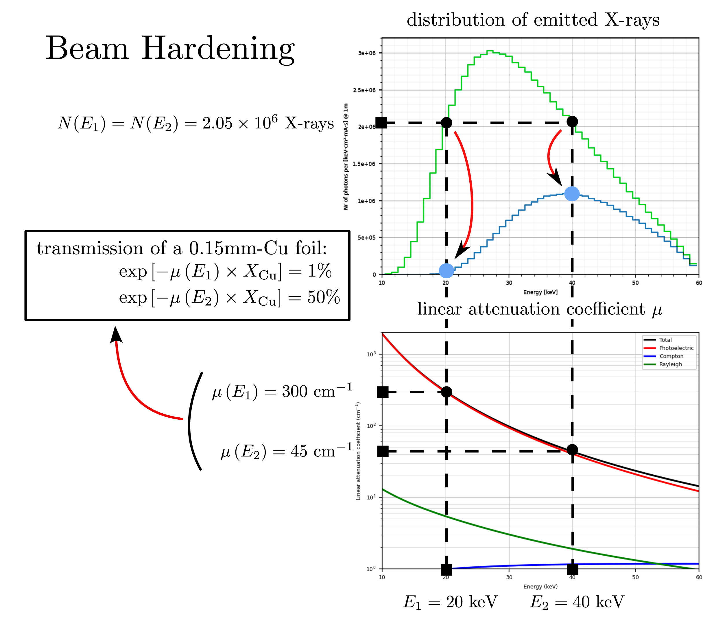
Fig. 91 Beam-hardening: stronger attenuation of x-ray with low energy

The signal measured \(I\left(p\right)\) by the flat panel detector is proportional to the deposited energy in the active area of the pixel \(p=\left(x,y\right)\). Assuming there are \(M\) different materials crossed by the x-rays from the source to pixel \(p\), the image \(I\left(p\right)\) can be modeled as follows:

\[ I\left(p\right) = \int_{E \in \mathrm{spectrum}} D\left(E,p\right) N_0\left(E,p\right) \exp\left( -\sum_{m=1}^M \mu_m\left(E\right) X_m\left(p\right) \right) \mathrm{d}E \]

where \(E\) is the photon energy, \(D\left(E,p\right)\) is the detector response, \(N_0\left(E,p\right)\) the number of photons emitted by the source, \(\mu_m\left(E\right)\) the linear attenuation coefficient of material \(m\) and \(X_m\left(p\right)\) the corresponding material thickness. If we have an homogeneous material \(M\) this boils down to

\[ I\left(p\right) = \int_{E \in spectrum} D\left(E\right) N_0\left(E,p\right) \exp\left( -\mu_M\left(E\right) X_M\left(p\right) \right) \mathrm{d}E \]

We can see that since the primary spectrum is not monochromatic the measurement is the sum of several attenuation laws. We could however compute the effective monochromatic attenuation that would give the same measurement:

\[ I\left(p\right) = I_0\left(p\right) \exp\left( -\sum_{m=1}^M \mu_m\left(E_{\mathrm{eff}}\right) X_m\left(p\right) \right) \]

with

\[ I_0\left(p\right) = \int_{E \in \mathrm{spectrum}} D\left(E,p\right) N_0\left(E,p\right) \mathrm{d}E \]

where $E_{\mathrm{eff}} corresponds to the monochromatic energy that would give the same attenuation than the one measured.

Mean energy:

• 31.6 keV (60 kV)

• 34.7 keV (+1.08 mm Al)

• 37.7 keV (+1.73 mm Al)

• 40.3 keV (+2.51 mm Al)

• 42.6 keV (+3.32 mm Al)

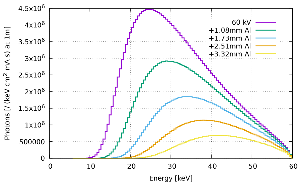
Fig. 92 Beam-hardening & Half-Value Layer (HVL)

Illustration of beam hardening by adding successively layers of 1/2 attenuation (\ emph {HVL}) in aluminum. We notice that we need a \ emph {HVL} more and more important to stop half the photons, and that the average energy of the photons in the spectrum also increases.

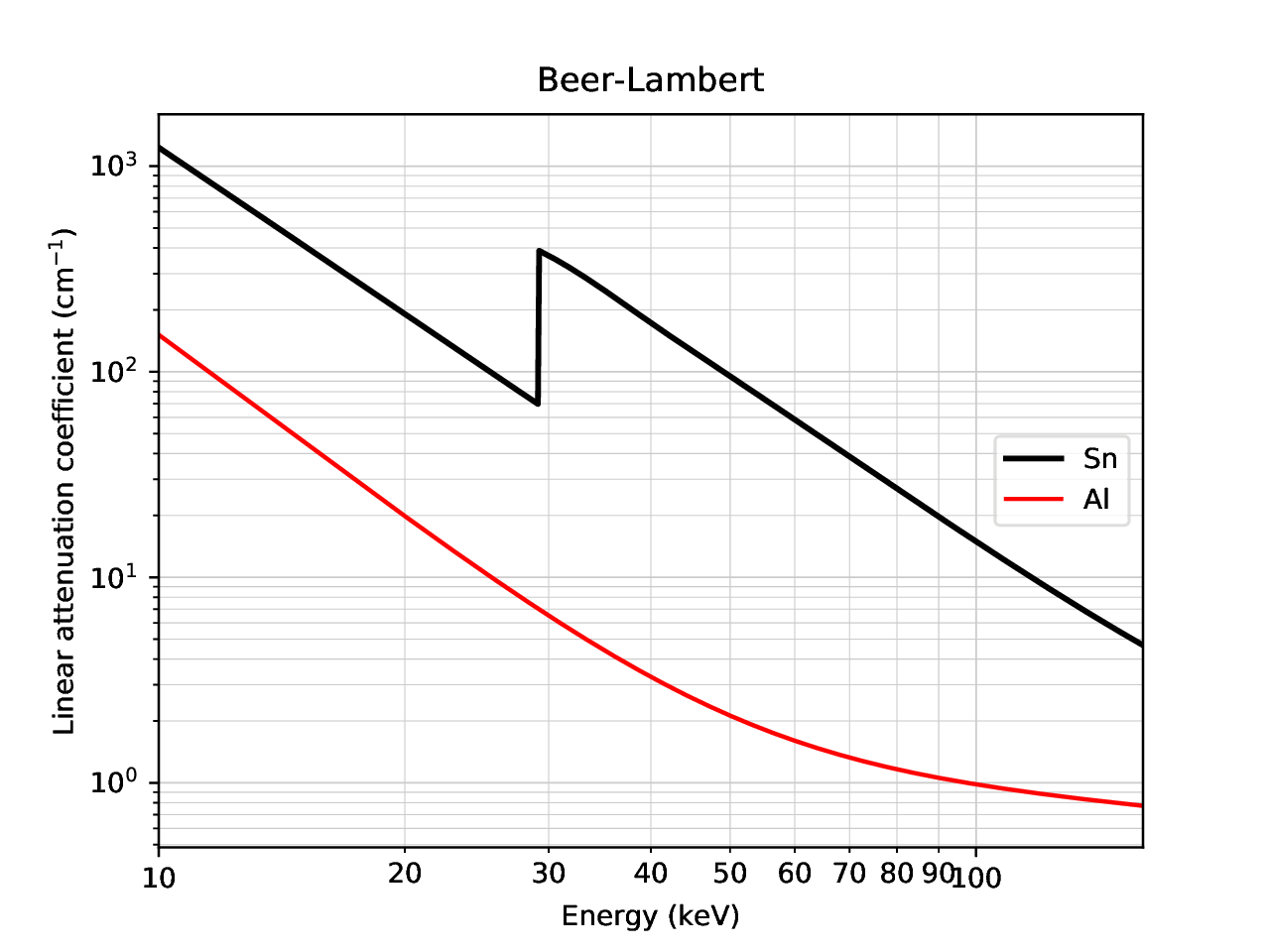
Fig. 93 Attenuation coefficients of the Al and Sn filters

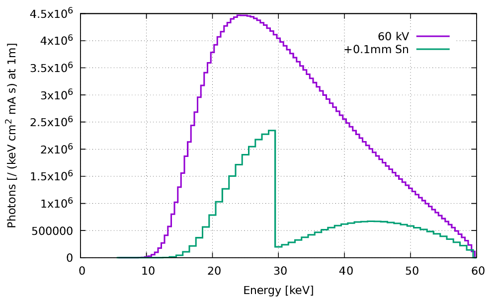
Fig. 94 Beam Shaping

When the material has no attenuation discontinuity in the energy range of the spectrum, such as aluminum previously, the transmitted spectrum is deformed but remains continued. On the other hand, the presence of discontinuity photoelectric, as here for tin, goes strongly modify the shape of the transmitted spectrum.

Standard characteristics

The radiative efficiency of the generator is very bad and the vast majority of electrical power is converted into heat at the anode. Summary of typical characteristics of X-rays.

• HT: \([20-800]\) kV

• Power: \(1\) W – \(5\) kW

• Focus: \(1\) micron – \(5\) mm

• Absorbed power \(= \text{kV} \times \text{mA}\)

• Radiative power \(\approx 10^{-6} \times Z \times \text{kV}^2 \times \text{mA}\) (NB : Bremsstrahlung slope \(\propto Z\))}

• Yield \(\approx 10^{-6} \times Z \times \text{kV}\) E.g. @ 60 kV (W anode): 99.5% heat, and 0.5% radiative

• mA \textit{vs} e-

\[ 1 \,\text{mA}\cdot\text{s} = 1 \,\text{mC} = \frac{1 \,\text{mC}}{1.6\times 10^{-19} \,\text{C}/\text{e-}} \,\text{e-} = 6.25\times 10^{15} \,\text{e-} \]

• Anode temperature (1 calorie = the amount of energy required to warm one gram of water from 19.5 to 20.5°C at standard atmospheric pressure)

\[ 100 \,\text{kV} \times 100 \,\text{mA} \times 10\,\text{s} = 10^5 \,\text{J} = 2.4 \times 10^4 \,\text{calorie} \]

The standard components of the generator are: the high-voltage transformer(s), the x-ray tube, the high-voltage cable and the controller (for the setting of high-voltage and current).

Fig. 95 System elements of an x-ray generator

Linear accelerator

Beyond 450 kV, it becomes difficult to accelerate electrons by a single high voltage. So it is necessary to accelerate them in successive stages for the bring to the desired energy. This is the principle of the linear accelerator which can deliver x-rays of several MeV. These energies are needed as soon as the thickness to be traversed exceeds a few centimeters of metal.

Fig. 96 Radiographic setup with linac

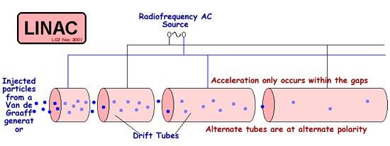
Fig. 97 Linear accelerator (linac) principle

Radioactive sources

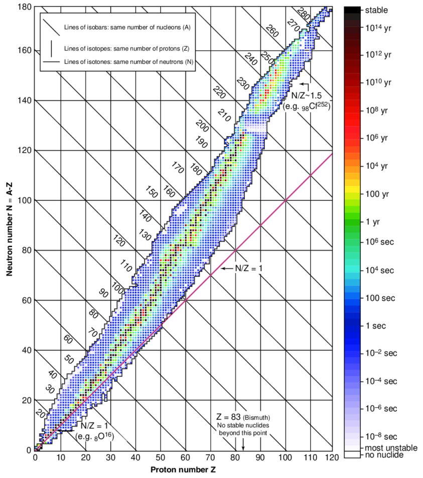
Fig. 98 Nuclides and stability

Detectors

Films and Image Intensifiers

Analog films were used initially. Flexible, they can tackle the pipes, but require a chemical process of development. More versions modern non-sensitive to ambient light are used for quality assurance of beams in radiotherapy.

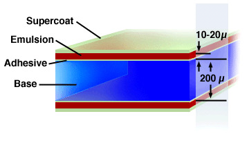
Fig. 99 Structure of a double emulsion film

Fig. 100 Radiographic testing with films

The photostimulable plates have the same function as the silver films but are reusable and do not require no chemical process.

Fig. 101 Example of plates

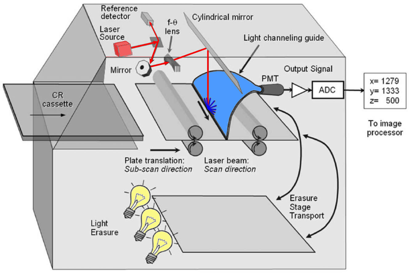
Fig. 102 Computed radiography: phosphor plates

Image intensifiers have long allowed to perform dynamic real-time imagery. They present very good resistance to radiation.

Flat panels

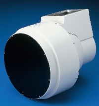
Fig. 103 Example of II

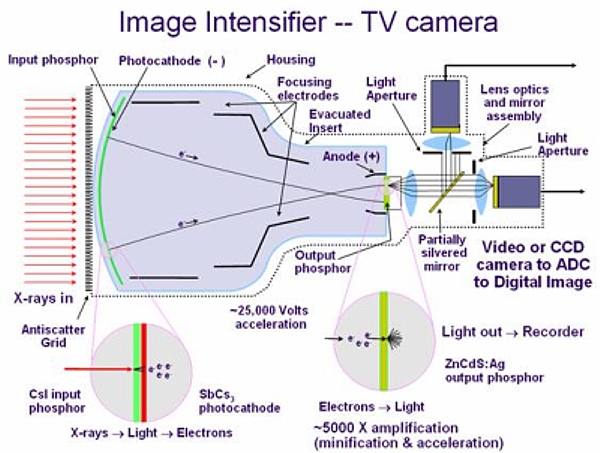
Fig. 104 Image intensifiers (II): Principle

Flat screens are now the benchmark in digital X-ray imaging. The reading electronics being in the field irradiation, special precautions should be taken to protect it. Two technologies exist: either indirect by the conversion into optical photons in the so-called scintillator material (thanks to a particular doping which allows to have a visible fluorescence following the effect photoelectric), or direct using the electrons expelled as a result of interactions in the detector (but this requires electrodes at each pixel). The vast majority of detectors are in integration, without the possibility of photon counting (because this requires a spectrometric chain at each pixel and a ultra fast electronics).

Fig. 105 Example of flat panel

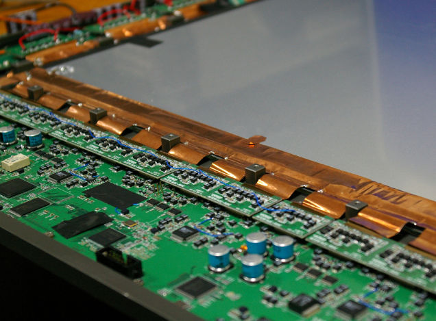
Fig. 106 Close-up on the readout electronics.

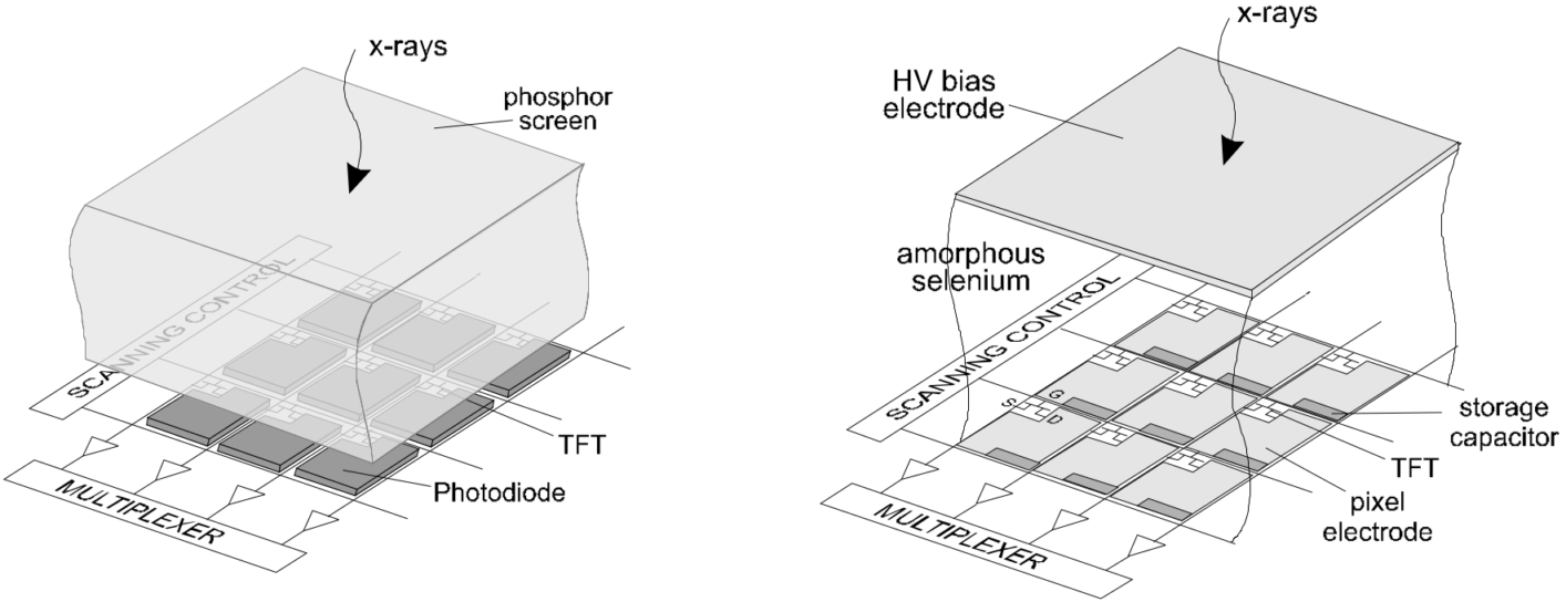
Fig. 107 Indirect (left) or direct (right) x-ray detetion setup. When indirect, explused electrons from x-ray interations are converted in optical photons, which in turn are read by photodiods. When indirect, electrons are directy read by electrodes.

Standard characteristics

Characteristics:

• Mode: integrating

  • Readout: 1-100 FPS

  • Pixel sizes: 1-1000 microns

  • Dynamic range: 8-20 bits

  • \(< 20\) MPixels

• Mode: counting

  • Countrate: 2-200 Mcps / mm\(^2\)

  • Pixel sizes: 50-1000 microns

  • No. of threshold: 1-100 (typ. 4)

  • \(< 1\) MPixels

• Geometry: flat panel or linear

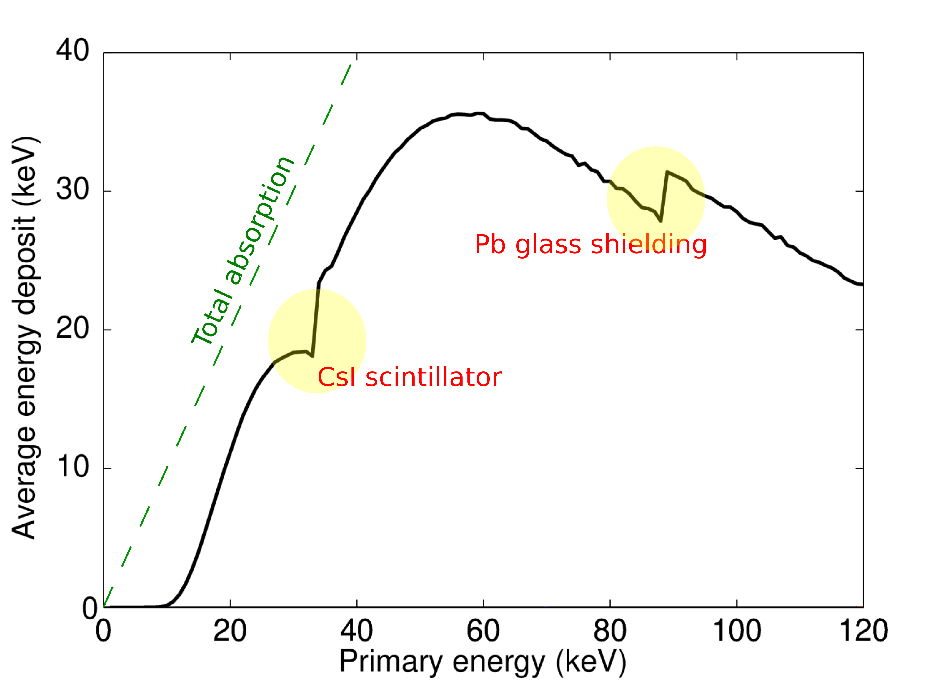
Fig. 108 Typical energy response of a x-ray flat panel

The typical energy response of some flat screen in the market is given in Fig. 108. At low energy, interactions are very probable and the detector has a response close to 100%, ie total absorption. When the energy is too great, X-rays pass through without interacting in the detector, which drop efficiency. Note the discontinuity of the CsI scintillator screen absorption (\(K_{\alpha}\) edge is \(33\) keV for I and \(36\) keV for Cs) and of the lead-glass shielding (\(K_{\alpha}\) edge is \(88\) keV for Pb).

Optical coupling

Fig. 109 Tandem lenses + \(\pi/4\) mirror

Fig. 110 Optic fibers

The protection of the reading electronics against radiation requires optical coupling solutions remote, with a tandem optic (as in Fig. 109) or a bundle of fibers (as in Fig. 110), but this lowers the detection efficiency compared to a flat screen for which the solid angle for the photodiodes is close to \(2\pi\) sr.

Fig. 111 shows the simplified architecture at the level of a pixel to get the x-ray energy spectrum and not a single integral scalar value.

Photon counting

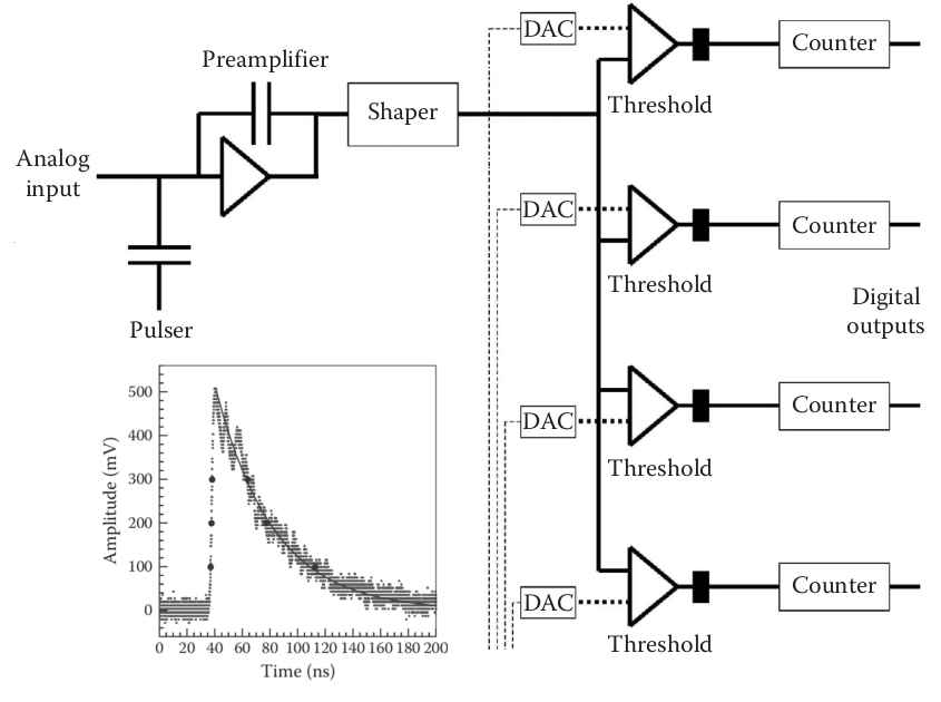
Fig. 111 Basic architecture of an individual pixel detection channel in the ASICs. From Iwanczyk DOI

The temporal response of a single photon is relatively long (several tens of ns), which can quickly pose stacking problems if the photon flux is too much important (see Fig. 112): this phenomenom is called pile-up. Charge sharing of a single photon deposit between neighboring pixels may also occur, which results in the detection of several photons of lower energy.

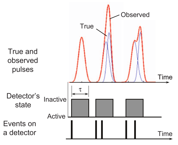
Fig. 112 Each photon incident on a detector will generate a pulse whose height is associated with the photon energy. Quasico- incident photons within the detector deadtime \(\tau\) are counted as \(1\) event with different energies from the originals due to pulse pileup effects. The former will result in lost counts and the latter in a distorted recorded energy spectrum. From Taguchi MP 2013 DOI

A photon does not necessarily deposit all of its energy: this is only the case if there is interaction by effect photoelectric. During a Compton interaction only one fraction of its energy is deposited: how to go up then to the incident energy of the photon if we want to have the energy distribution? X-ray “color” imaging is not easy to master. Fig. 113 shows the detected radiation spectrum of \(^{22}_{11}\mathsf{Na} \Rightarrow ~^{22}_{10}\mathsf{Ne} + (180.8{\%}) \beta^+ + (99.9{\%}) \gamma_{1.27\mathsf{MeV}}\).

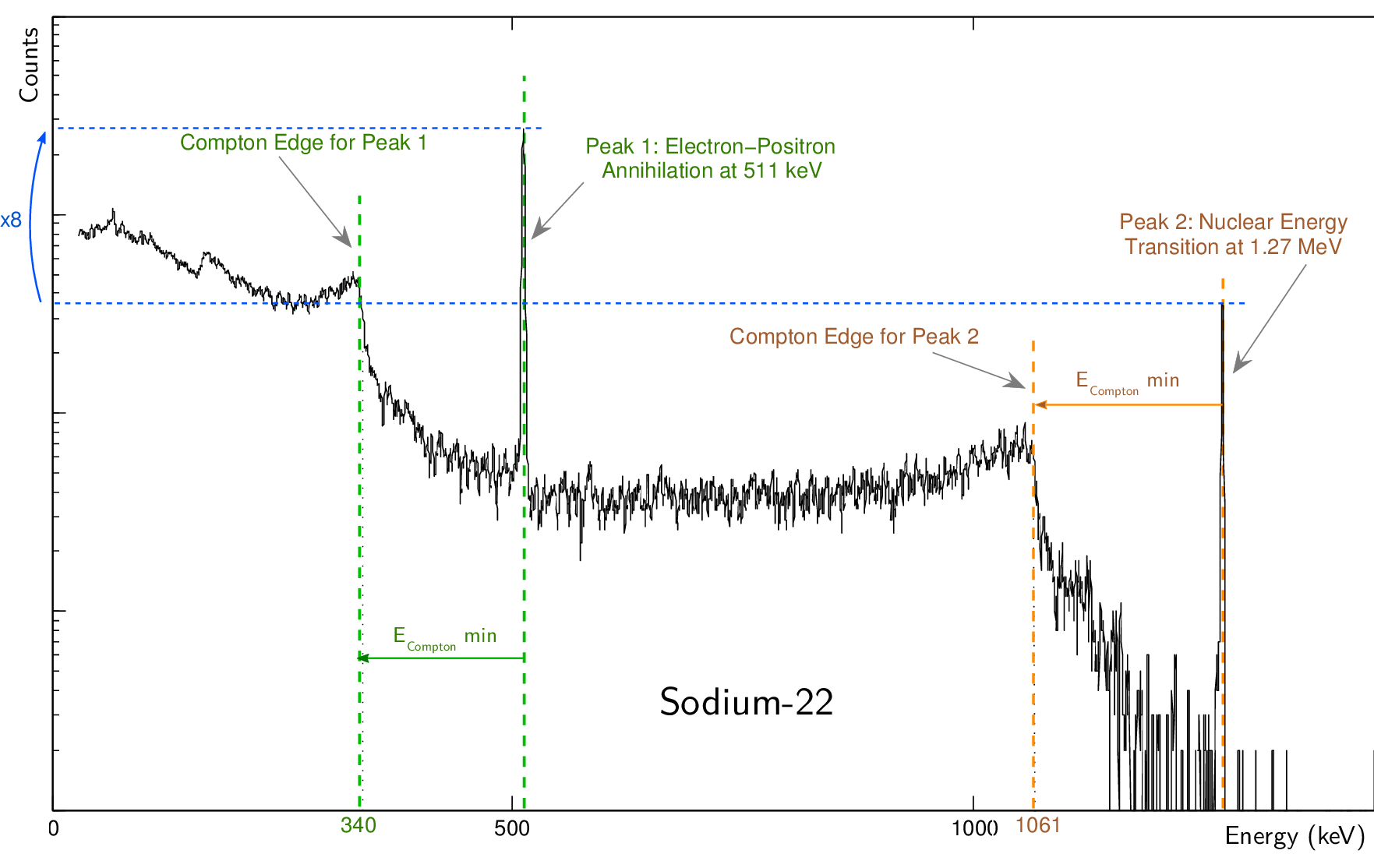
Fig. 113 Absorbed energy spectrum of the desexcitation radiations of Na-22. Only 2 energy lines should be visible: one at 511keV of intensity twce the one one at 1.27 MeV.

The detected spectrum would be the incident emitted one if all photons had deposited all their energy by photoelectric effect. Instead, many photons did interact by Compton scattering and only part of their energy was deposied in the detector: the maximum energy deposition by the Compton electron is when \(\theta=\pi\), which is called the Compton edge (see Fig. 113).

Flat Field

X-ray detectors have the same characteristics and limits than standard imaging systems: afterglow, the dynamics of digitization, spatial heterogeneities and temporal… Normalization by an objectless image (flat field) corrects a part of the artifacts.

• Scatter sensitivity \(\Rightarrow\) slot-scanning vs flat panel

• Veiling glare due to secondary energy carriers (optical photons or e\(^-\)) \(\Rightarrow\) drop at low frequencies

• Dynamic range

• Spatial artifacts \(\Rightarrow\) defective pixel map

• Temporal artifacts \(\Rightarrow\) lag (residual signal), flicking pixels

• Temporal stability \(\Rightarrow\) varying performances over time

The image formation process may therefore be approximated as follows for a mono-material and mono-energy:

\[ I_{\mathsf{Object}}\left(p\right) = I_{\mathsf{Source}}\left(p\right) R_{\mathsf{Detector}}\left(p\right) \exp\left[-\mu\left(p\right) X\left(p\right)\right] + I_{\mathsf{Dark}}\left(p\right) \]

where \(p\) is the pixel, \(I_{\mathsf{Source}}\) the x-rays emitted by the source, \(R_{\mathsf{Detector}}\) the detector response, \(\mu\) the effective attenuation coefficient, \(X\) the material thickness, and \(I_{\mathsf{Dark}}\) the dark current. The flattening makes it possible to cope with those spatial variations of x-ray emission and detector response.

Parameters

• \(I_\mathsf{Image}\): acquisition with object

• \(I_\mathsf{Dark}\): acquisition without radiation

• \(I_\mathsf{White}\): acquisition without object

Flattening

\[ I_\mathsf{Flat~Image}\left(p\right) = \frac{I_\mathsf{Object}\left(p\right) - I_\mathsf{Dark}\left(p\right)}{I_\mathsf{White}\left(p\right) - I_\mathsf{Dark}\left(p\right)} \]

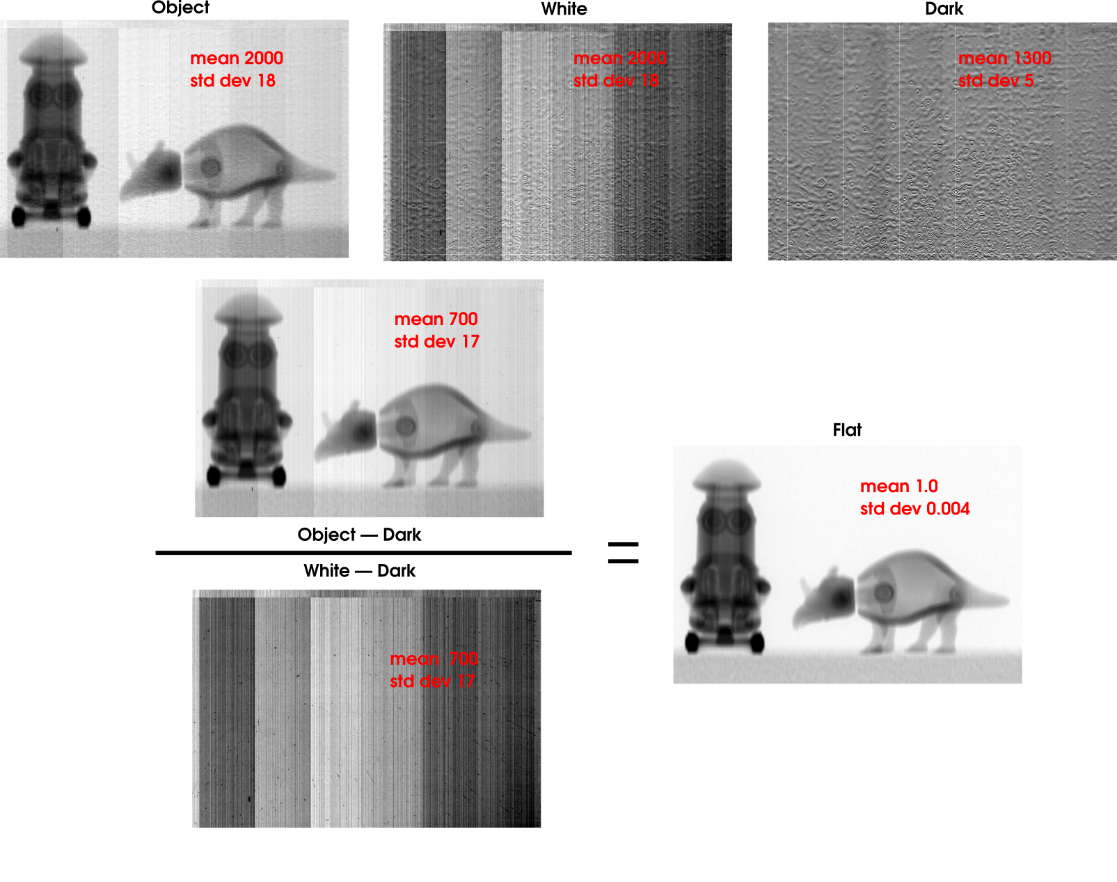
Fig. 114 Example of flat-field

Magnification & Unsharpness

The x-ray image is a projection of the attenuation and the size of the projection image is larger than the size of the object: there is a magnification \(M \geq 1\) which can be measured as the ration of the source-to-detector distance over the source-to-object distance (see image Fig. 115):

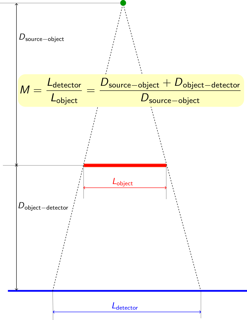
Fig. 115 Geometric magnification

The blurring in image X has two causes: the detector itself (the inherent unsharpnness) and the non-punctuality of the source of radiation (geometric unsharpness). If the focal task of the source is oriented, the geometric unsharpness may depend on the position on the detector.

Parameters

• \(u^2_{\mathsf{geometrical}}\): unsharpness due to the source extent

• \(u^2_{\mathsf{inherent}}\): unsharpness due to the detector spatial response

Total unsharpness \(u^2_{\mathsf{total}}\)

\[ u^2_{\mathsf{total}} = u^2_{\mathsf{geometrical}} + u^2_{\mathsf{inherent}} \]

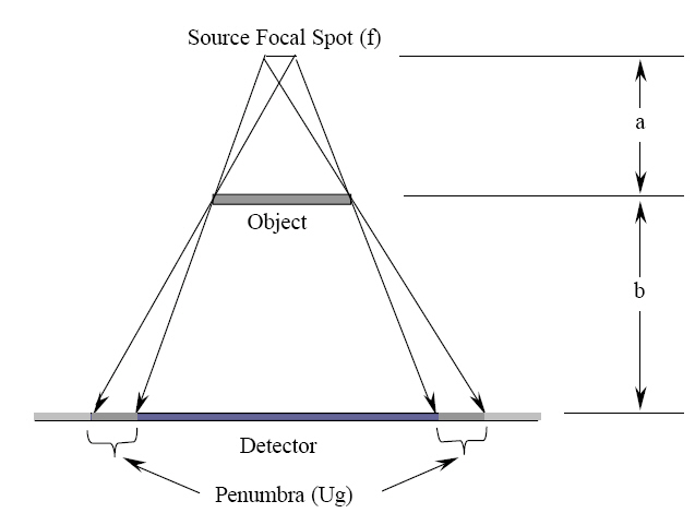
Fig. 116 Geometric unsharpness

The geometric unsharpness is directly related to the source size \(f\) up to the magnification \(M\)as Fig. 116 shows. Note that an angled anode generated a space-variant geometric unsharpness.

\[ u_{\mathsf{geometrical}} = \frac{b}{a} f = (M-1) f \]

where, given the notation of figure Fig. 116, the magnification \(M\) is given by

\[ M = \frac{a+b}{a} \]

The inherent unsharpness, also named point-spread function (PSF), depends on the detector technology (direct or inidrect), the scintillator (if indirect) thickness, the coating and mounting materials, the incident photon energy…

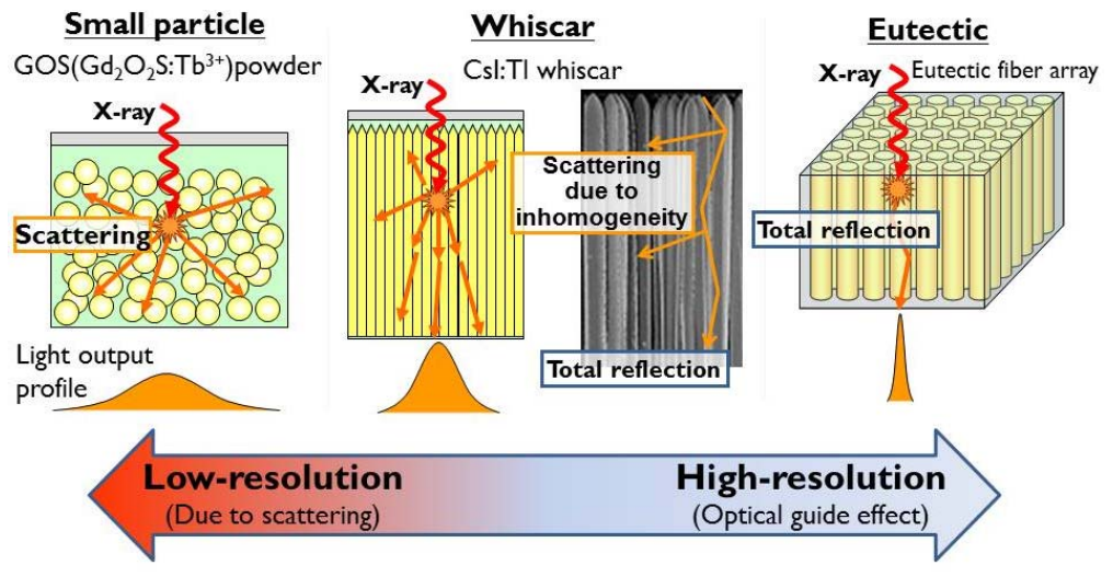
Fig. 117 Expected point spread function (PSF) of three kinds of material state. Small particle gives low resolution due to scattering. Whisker gives higher resolution than that of particles. Highest resolution is expected by the eutectic with optical guide effect. From Dujardin TNS 2018 DOI

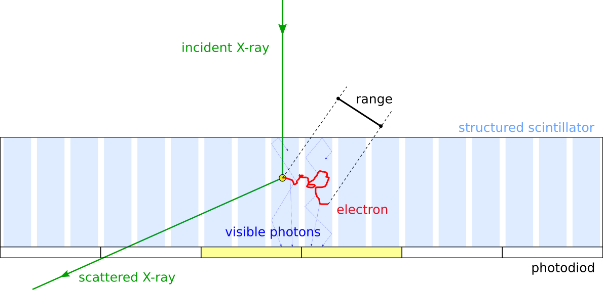
Fig. 118 When an X-ray interacts with the scintillator, the electron delocalizes the information and produces optical photons all along its range. Therefore several neighboring pixels (photodiods) can be hit for a single X-ray event. The detector unsharpness is thus related to the incident x-ray energy.

Image primitives

SNR, CNR and SPR

The contrast between two areas of the RX image is directly linked to the law of attenuation. A change in current or the generator voltage will directly impact it (modification of \(I_0\) and \(\mu\). Alone, contrast is not enough not to characterize the detectability, it is necessary to take a measurement related to noise in the radiograph. The presence of secondary radiation from interactions (scattered, fluorescence…) will also degrade the dynamics.

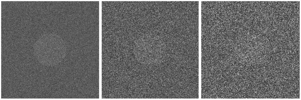
Fig. 119 The ability to detect an object is dependent upon both the contrast of the object and the noise in the image. From Dance IAEA

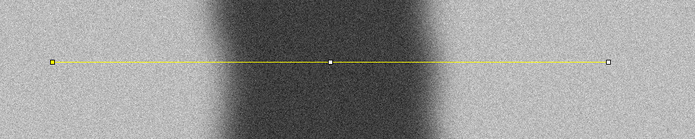
Fig. 120 Example of image with noise. The profile in figure Fig. 121 is sampled along the yellow line.

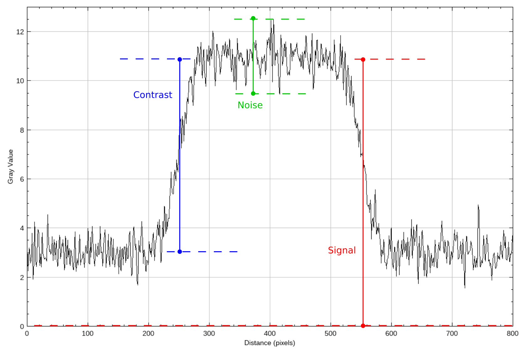
Fig. 121 Notions of signal, contrast and noise in an image. The profile has been sampled along the yellow line in figure Fig. 120.

Image primitives

• Absolute contrast

\[ C = I_0 - I_1 = I_0 \left(1 - \exp(-\mu T)\right) \]

• Relative contrast

\[ C_{\%} = \frac{I_0 - I_1}{I_0} = 1 - \exp(-\mu T) \]

• Counting process: Poisson noise (mean = variance) for the nr of photons

\[ \mathsf{SNR} = \frac{\mbox{mean}}{\sqrt{\mbox{variance}}} = \frac{N}{\sqrt{N}} = \sqrt{N} \]

• SPR: Scatter-to-Primary Ratio

\[ \mathsf{SPR} = \frac{\text{Contribution due to secondary (scattered mainly) photons}}{\text{Contribution due the primary (ie without interaction) photons}} \]

• Nota Bene: remind that the generator settings (mA, s & kV) influence those primitives

MTF and DQE

The contrast in the image also depends on the content spatial frequency of the object. The transfer function of modulation (MTF) makes it possible to characterize the evolution of contrast with the spatial frequency.

Fig. 122 shows a typical bar-pattern test object to assess the spatial resolution. It ia usually made of lead and PMMA. The higher the spatial frequency the lower the intensity contrast.

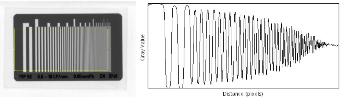
Fig. 122 X-ray resolution bar pattern with increasing frequencies (left) and horizontal intensity profile extracted fro the image (right).

The drop of intensity contrast with respect to the spatial frequency is observed in Fig. 123.

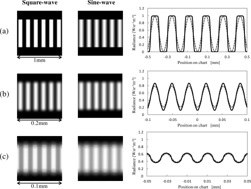
Fig. 123 Illustration of the image blurring from increasing spatial frequencies.

The MTF value at frequency \(f\) is simply computed from the contrast ratio with respect to the contrast when the frequency tends to \(0\).

\[ \text{MTF} (f) = \frac{[\text{Max}-\text{Min}](f)}{\lim_{\nu\rightarrow 0}[\text{Max}-\text{Min}](\nu)} \]

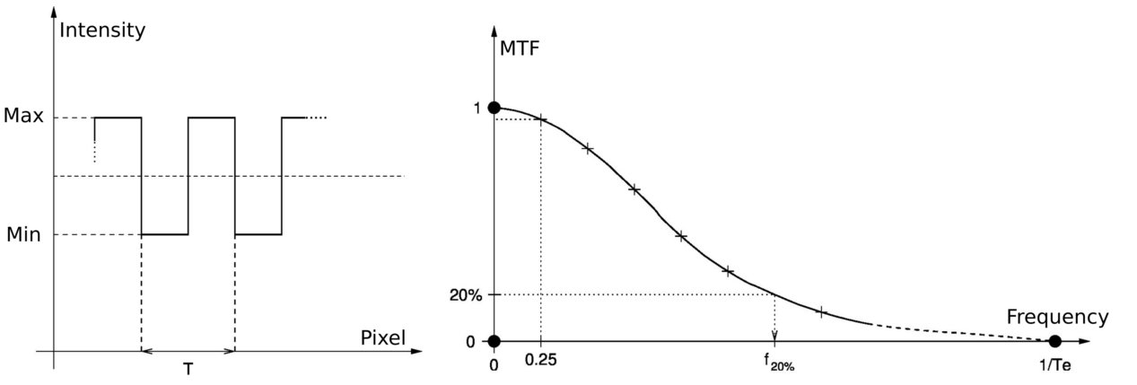
Fig. 124 Typical intensity profile of a bar pattern on a image (left) and the corresponding MTF.

The ratio of the MTF to the noise power spectrum (NPS) gives the quantum detection efficiency (DQE), which ultimately represents a contrast on noise as a function of the spatial frequency.

\[ DQE (\nu) = \frac{\mathsf{SNR}^2_{\mathsf{out}}(\nu)}{\mathsf{SNR}^2_{\mathsf{in}}(\nu)} \]

we have

\[ \mathsf{SNR}^2_{\mathsf{in}}(\nu) = \left(\frac{N_0}{\sqrt{N_0}}\right)^2 = N_0 \]

with \(N_0\) in [#phots~mm\(^{-2}\)] for a given exposure. Then

\[ DQE (\nu) = \frac{\mathsf{MTF}^2(\nu)}{N_{0} \; \mathsf{NPS}(\nu)} \]

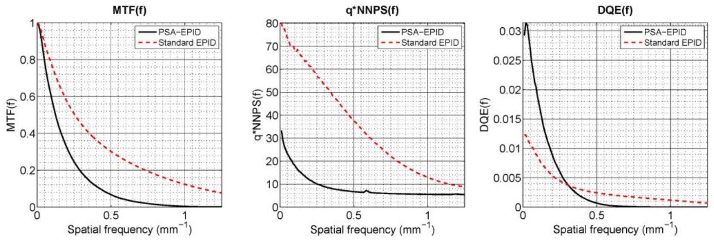
Fig. 125 Comparison of the experimentally measured MTF, qNNPS and DQE for two portable imaging devices (EPID) which are similar to flat panels: a prototype PSA-EPID and a standard phosphor-based EPID. From Blake MP 2018 DOI

Nota Bene: the patient (scattering, magnification…) is now being taken into account to compute effective figures of merit.

Moiré or aliasing can also occur in X-ray imaging. It is directly related to the spatial sampling of the detector, ie the size of the pixel.

Fig. 126 Effect of undersampling: Moiré patterns or aliasing

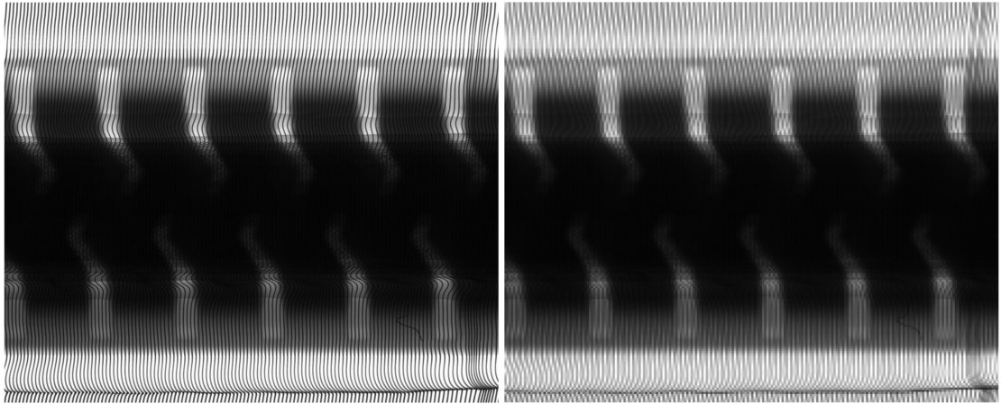
Fig. 127 X-ray radiography of a tyre with a small pixel size (left) and a 8-times larger pixel size (right). Moiré (aliasing patterns are clearly visible.